Notebook: using jsonstat.py with eurostat api¶

This Jupyter notebook shows the python library jsonstat.py in action. It shows how to explore dataset downloaded from a data provider. This notebook uses some datasets from Eurostat. Eurostat provides a rest api to download its datasets. You can find details about the api here It is possible to use a query builder for discovering the rest api parameters. The following image shows the query builder:

# all import here
from __future__ import print_function
import os
import pandas as pd
import jsonstat

import matplotlib as plt
%matplotlib inline

1 - Exploring data with one dimension (time) with size > 1¶

Following cell downloads a datataset from eurostat. If the file is already downloaded use the copy presents on the disk. Caching file is useful to avoid downloading dataset every time notebook runs. Caching can speed the development, and provides consistent results. You can see the raw data here

url_1 = 'http://ec.europa.eu/eurostat/wdds/rest/data/v1.1/json/en/nama_gdp_c?precision=1&geo=IT&unit=EUR_HAB&indic_na=B1GM'
file_name_1 = "eurostat-name_gpd_c-geo_IT.json"

file_path_1 = os.path.abspath(os.path.join("..", "tests", "fixtures", "www.ec.europa.eu_eurostat", file_name_1))
if os.path.exists(file_path_1):
    print("using already donwloaded file {}".format(file_path_1))
else:
    print("download file")
    jsonstat.download(url_1, file_name_1)
    file_path_1 = file_name_1

using already donwloaded file /Users/26fe_nas/gioprj.on_mac/prj.python/jsonstat.py/tests/fixtures/www.ec.europa.eu_eurostat/eurostat-name_gpd_c-geo_IT.json

Initialize JsonStatCollection with eurostat data and print some info about the collection.

collection_1 = jsonstat.from_file(file_path_1)
collection_1

JsonstatCollection contains the following JsonStatDataSet:

pos	dataset
0	'nama_gdp_c'

Previous collection contains only a dataset named ‘nama_gdp_c‘

nama_gdp_c_1 = collection_1.dataset('nama_gdp_c')
nama_gdp_c_1

name: 'nama_gdp_c'
title: 'GDP and main components - Current prices'
size: 4

pos	id	label	size	role
0	unit	unit	1
1	indic_na	indic_na	1
2	geo	geo	1
3	time	time	69

All dimensions of the dataset ‘nama_gdp_c‘ are of size 1 with exception of time dimension. Let’s explore the time dimension.

nama_gdp_c_1.dimension('time')

pos	idx	label
0	'1946'	'1946'
1	'1947'	'1947'
2	'1948'	'1948'
3	'1949'	'1949'
...	...	...

Get value for year 2012.

nama_gdp_c_1.value(time='2012')

Convert the jsonstat data into a pandas dataframe.

df_1 = nama_gdp_c_1.to_data_frame('time', content='id')
df_1.tail()

	unit	indic_na	geo	Value
time
2010	EUR_HAB	B1GM	IT	25700.0
2011	EUR_HAB	B1GM	IT	26000.0
2012	EUR_HAB	B1GM	IT	25700.0
2013	EUR_HAB	B1GM	IT	25600.0
2014	EUR_HAB	B1GM	IT	NaN

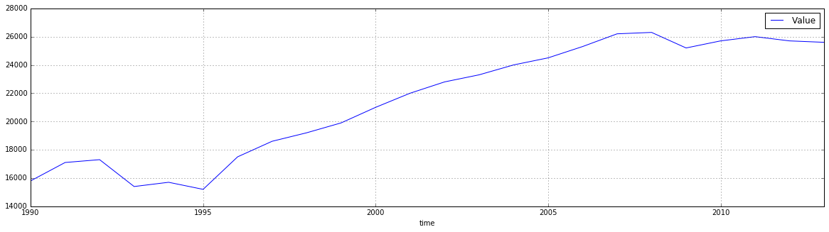
Adding a simple plot

df_1 = df_1.dropna() # remove rows with NaN values
df_1.plot(grid=True, figsize=(20,5))

<matplotlib.axes._subplots.AxesSubplot at 0x114bc12b0>

2 - Exploring data with two dimensions (geo, time) with size > 1¶

Download or use the jsonstat file cached on disk. The cache is used to avoid internet download during the devolopment to make the things a bit faster. You can see the raw data here

url_2 = 'http://ec.europa.eu/eurostat/wdds/rest/data/v1.1/json/en/nama_gdp_c?precision=1&geo=IT&geo=FR&unit=EUR_HAB&indic_na=B1GM'
file_name_2 = "eurostat-name_gpd_c-geo_IT_FR.json"

file_path_2 = os.path.abspath(os.path.join("..", "tests", "fixtures", "www.ec.europa.eu_eurostat", file_name_2))
if os.path.exists(file_path_2):
    print("using alredy donwloaded file {}".format(file_path_2))
else:
    print("download file and storing on disk")
    jsonstat.download(url, file_name_2)
    file_path_2 = file_name_2

using alredy donwloaded file /Users/26fe_nas/gioprj.on_mac/prj.python/jsonstat.py/tests/fixtures/www.ec.europa.eu_eurostat/eurostat-name_gpd_c-geo_IT_FR.json

collection_2 = jsonstat.from_file(file_path_2)
nama_gdp_c_2 = collection_2.dataset('nama_gdp_c')
nama_gdp_c_2

name: 'nama_gdp_c'
title: 'GDP and main components - Current prices'
size: 4

pos	id	label	size	role
0	unit	unit	1
1	indic_na	indic_na	1
2	geo	geo	2
3	time	time	69

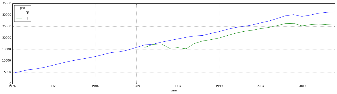
nama_gdp_c_2.dimension('geo')

pos	idx	label
0	'FR'	'France'
1	'IT'	'Italy'

nama_gdp_c_2.value(time='2012',geo='IT')

nama_gdp_c_2.value(time='2012',geo='FR')

df_2 = nama_gdp_c_2.to_table(content='id',rtype=pd.DataFrame)
df_2.tail()

	unit	indic_na	geo	time	Value
133	EUR_HAB	B1GM	IT	2010	25700.0
134	EUR_HAB	B1GM	IT	2011	26000.0
135	EUR_HAB	B1GM	IT	2012	25700.0
136	EUR_HAB	B1GM	IT	2013	25600.0
137	EUR_HAB	B1GM	IT	2014	NaN

df_FR_IT = df_2.dropna()[['time', 'geo', 'Value']]
df_FR_IT = df_FR_IT.pivot('time', 'geo', 'Value')
df_FR_IT.plot(grid=True, figsize=(20,5))

<matplotlib.axes._subplots.AxesSubplot at 0x114c0f0b8>

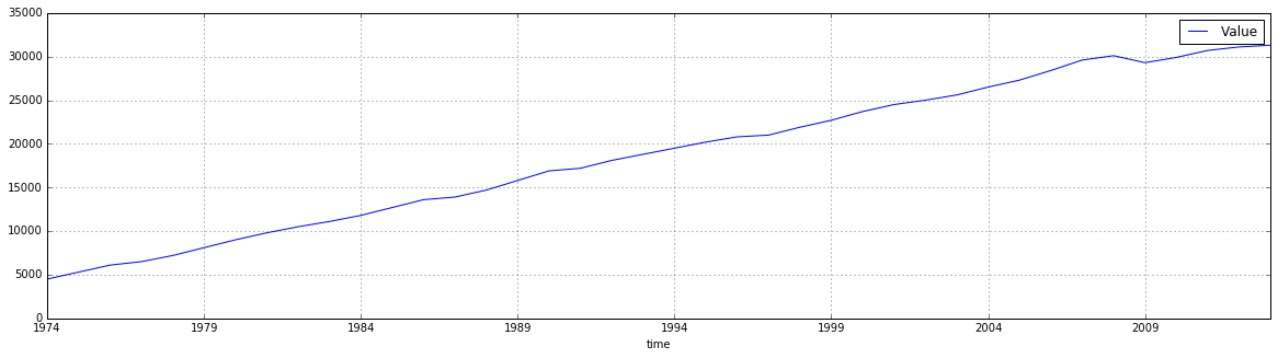
df_3 = nama_gdp_c_2.to_data_frame('time', content='id', blocked_dims={'geo':'FR'})
df_3 = df_3.dropna()
df_3.plot(grid=True,figsize=(20,5))

<matplotlib.axes._subplots.AxesSubplot at 0x1178e7d30>

df_4 = nama_gdp_c_2.to_data_frame('time', content='id', blocked_dims={'geo':'IT'})
df_4 = df_4.dropna()
df_4.plot(grid=True,figsize=(20,5))

<matplotlib.axes._subplots.AxesSubplot at 0x117947630>