Using istat api
Next step is to set a cache dir where to store json files downloaded
from Istat. Storing file on disk speeds up development, and assures
consistent results over time. Eventually, you can delete donwloaded
files to get a fresh copy.
cache_dir = os.path.abspath(os.path.join("..", "tmp", "istat_cached")) # you could choice /tmp
istat.cache_dir(cache_dir)
print("cache_dir is '{}'".format(istat.cache_dir()))
cache_dir is '/Users/26fe_nas/gioprj.on_mac/prj.python/jsonstat.py/tmp/istat_cached'
List all istat areas
| id | desc |
|---|
| 3 | 2011 Population and housing census |
| 4 | Enterprises |
| 7 | Environment and Energy |
| 8 | Population and Households |
| 9 | Households Economic Conditions and Disparities |
| 10 | Health statistics |
| 11 | Social Security and Welfare |
| 12 | Education and training |
| 13 | Communication, culture and leisure |
| 14 | Justice and Security |
| 15 | Citizens' opinions and satisfaction with life |
| 16 | Social participation |
| 17 | National Accounts |
| 19 | Agriculture |
| 20 | Industry and Construction |
| 21 | Services |
| 22 | Public Administrations and Private Institutions |
| 24 | External Trade and Internationalisation |
| 25 | Prices |
| 26 | Labour |
List all datasets contained into area LAB (Labour)
istat_area_lab = istat.area('LAB')
istat_area_lab
IstatArea: cod = LAB description = Labour
List all dimension for dataset DCCV_TAXDISOCCU (Unemployment rate)
istat_dataset_taxdisoccu = istat_area_lab.dataset('DCCV_TAXDISOCCU')
istat_dataset_taxdisoccu
DCCV_TAXDISOCCU(9):Unemployment rate
| nr | name | nr. values | values (first 3 values) |
|---|
| 0 | Territory | 136 | 1:'Italy', 3:'Nord', 4:'Nord-ovest' ... |
| 1 | Data type | 1 | 6:'unemployment rate' |
| 2 | Measure | 1 | 1:'percentage values' |
| 3 | Gender | 3 | 1:'males', 2:'females', 3:'total' ... |
| 4 | Age class | 14 | 32:'18-29 years', 3:'20-24 years', 4:'15-24 years' ... |
| 5 | Highest level of education attained | 5 | 11:'tertiary (university, doctoral and specialization courses)', 12:'total', 3:'primary school certificate, no educational degree' ... |
| 6 | Citizenship | 3 | 1:'italian', 2:'foreign', 3:'total' ... |
| 7 | Duration of unemployment | 2 | 2:'12 months and more', 3:'total' |
| 8 | Time and frequency | 193 | 1536:'Q4-1980', 2049:'Q4-2007', 1540:'1981' ... |
Extract data from dataset DCCV_TAXDISOCCU
spec = {
    "Territory": 0,                            # 1 Italy
    "Data type": 6,                            # (6:'unemployment rate')
    'Measure': 1,                              # 1 : 'percentage values'
    'Gender': 3,                               # 3 total
    'Age class':31,                            # 31:'15-74 years'
    'Highest level of education attained': 12, # 12:'total',
    'Citizenship': 3,                          # 3:'total')
    'Duration of unemployment': 3,             # 3:'total'
    'Time and frequency': 0                    # All
}

# convert istat dataset into jsonstat collection and print some info
collection = istat_dataset_taxdisoccu.getvalues(spec)
collection
JsonstatCollection contains the following JsonStatDataSet:
| pos | dataset |
| 0 | 'IDITTER107*IDTIME' |
Print some info of the only dataset contained into the above jsonstat
collection
jsonstat_dataset = collection.dataset(0)
jsonstat_dataset
name: 'IDITTER107*IDTIME'label: 'Unemployment rate by Territory and Time and frequency - unemployment rate - percentage values - 15-74 years'size: 7830
| pos | id | label | size | role |
| 0 | IDITTER107 | Territory | 135 | |
| 1 | IDTIME | Time and frequency | 58 | |
df_all = jsonstat_dataset.to_table(rtype=pd.DataFrame)
df_all.head()
|
Territory |
Time and frequency |
Value |
| 0 |
Italy |
2004 |
8.01 |
| 1 |
Italy |
Q1-2004 |
8.68 |
| 2 |
Italy |
Q2-2004 |
7.88 |
| 3 |
Italy |
Q3-2004 |
7.33 |
| 4 |
Italy |
Q4-2004 |
8.17 |
df_all.pivot('Territory', 'Time and frequency', 'Value').head()
| Time and frequency |
2004 |
2005 |
2006 |
2007 |
2008 |
2009 |
2010 |
2011 |
2012 |
2013 |
... |
Q4-2005 |
Q4-2006 |
Q4-2007 |
Q4-2008 |
Q4-2009 |
Q4-2010 |
Q4-2011 |
Q4-2012 |
Q4-2013 |
Q4-2014 |
| Territory |
|
|
|
|
|
|
|
|
|
|
|
|
|
|
|
|
|
|
|
|
|
| Abruzzo |
7.71 |
7.88 |
6.57 |
6.17 |
6.63 |
7.97 |
8.67 |
8.59 |
10.85 |
11.29 |
... |
6.95 |
6.84 |
5.87 |
6.67 |
7.02 |
9.15 |
9.48 |
10.48 |
11.21 |
12.08 |
| Agrigento |
20.18 |
17.62 |
13.40 |
16.91 |
16.72 |
17.43 |
19.42 |
17.61 |
19.48 |
20.98 |
... |
NaN |
NaN |
NaN |
NaN |
NaN |
NaN |
NaN |
NaN |
NaN |
NaN |
| Alessandria |
5.34 |
5.37 |
4.65 |
4.63 |
4.85 |
5.81 |
5.34 |
6.66 |
10.48 |
11.80 |
... |
NaN |
NaN |
NaN |
NaN |
NaN |
NaN |
NaN |
NaN |
NaN |
NaN |
| Ancona |
5.11 |
4.14 |
4.05 |
3.49 |
3.78 |
5.82 |
4.94 |
6.84 |
9.20 |
11.27 |
... |
NaN |
NaN |
NaN |
NaN |
NaN |
NaN |
NaN |
NaN |
NaN |
NaN |
| Arezzo |
4.55 |
5.50 |
4.88 |
4.61 |
4.91 |
5.51 |
5.87 |
6.04 |
7.33 |
8.04 |
... |
NaN |
NaN |
NaN |
NaN |
NaN |
NaN |
NaN |
NaN |
NaN |
NaN |
5 rows × 58 columns
spec = {
    "Territory": 1,                            # 1 Italy
    "Data type": 6,                            # (6:'unemployment rate')
    'Measure': 1,
    'Gender': 3,
    'Age class':0,                             # all classes
    'Highest level of education attained': 12, # 12:'total',
    'Citizenship': 3,                          # 3:'total')
    'Duration of unemployment': 3,             #  3:'total')
    'Time and frequency': 0                    # All
}

# convert istat dataset into jsonstat collection and print some info
collection_2 = istat_dataset_taxdisoccu.getvalues(spec)
collection_2
JsonstatCollection contains the following JsonStatDataSet:
| pos | dataset |
| 0 | 'IDCLASETA28*IDTIME' |
df = collection_2.dataset(0).to_table(rtype=pd.DataFrame, blocked_dims={'IDCLASETA28':'31'})
df.head(6)
|
Age class |
Time and frequency |
Value |
| 0 |
15-74 years |
Q4-1992 |
NaN |
| 1 |
15-74 years |
1993 |
NaN |
| 2 |
15-74 years |
Q1-1993 |
NaN |
| 3 |
15-74 years |
Q2-1993 |
NaN |
| 4 |
15-74 years |
Q3-1993 |
NaN |
| 5 |
15-74 years |
Q4-1993 |
NaN |
df = df.dropna()
df = df[df['Time and frequency'].str.contains(r'^Q.*')]
# df = df.set_index('Time and frequency')
df.head(6)
|
Age class |
Time and frequency |
Value |
| 57 |
15-74 years |
Q1-2004 |
8.68 |
| 58 |
15-74 years |
Q2-2004 |
7.88 |
| 59 |
15-74 years |
Q3-2004 |
7.33 |
| 60 |
15-74 years |
Q4-2004 |
8.17 |
| 62 |
15-74 years |
Q1-2005 |
8.27 |
| 63 |
15-74 years |
Q2-2005 |
7.54 |
df.plot(x='Time and frequency',y='Value', figsize=(18,4))
<matplotlib.axes._subplots.AxesSubplot at 0x1184b1908>
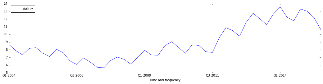
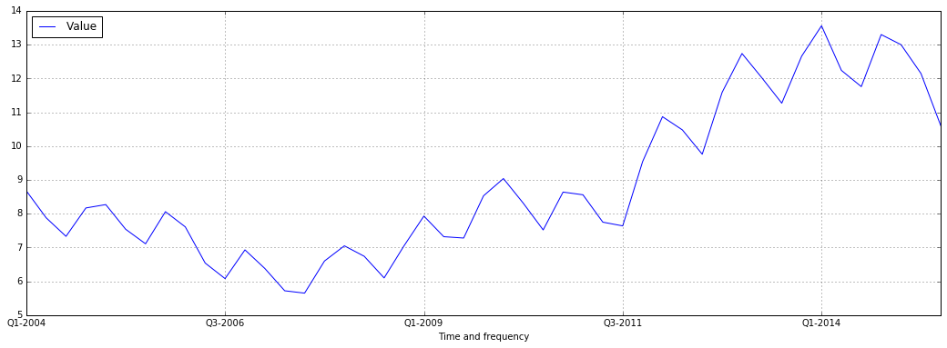
fig = plt.figure(figsize=(18,6))
ax = fig.add_subplot(111)
plt.grid(True)
df.plot(x='Time and frequency',y='Value', ax=ax, grid=True)
# kind='barh', , alpha=a, legend=False, color=customcmap,
# edgecolor='w', xlim=(0,max(df['population'])), title=ttl)
<matplotlib.axes._subplots.AxesSubplot at 0x11a898b70>
# plt.figure(figsize=(7,4))
# plt.plot(df['Time and frequency'],df['Value'], lw=1.5, label='1st')
# plt.plot(y[:,1], lw=1.5, label='2st')
# plt.plot(y,'ro')
# plt.grid(True)
# plt.legend(loc=0)
# plt.axis('tight')
# plt.xlabel('index')
# plt.ylabel('value')
# plt.title('a simple plot')
# forza lavoro
istat_forzlv = istat.dataset('LAB', 'DCCV_FORZLV')

spec = {
    "Territory": 'Italy',
    "Data type": 'number of labour force 15 years and more (thousands)',                            #
    'Measure':   'absolute values',
    'Gender':    'total',
    'Age class': '15 years and over',
    'Highest level of education attained': 'total',
    'Citizenship': 'total',
    'Time and frequency': 0
}

df_forzlv = istat_forzlv.getvalues(spec).dataset(0).to_table(rtype=pd.DataFrame)
df_forzlv = df_forzlv.dropna()
df_forzlv = df_forzlv[df_forzlv['Time and frequency'].str.contains(r'^Q.*')]
df_forzlv.tail(6)
|
Time and frequency |
Value |
| 187 |
Q2-2014 |
25419.15 |
| 188 |
Q3-2014 |
25373.70 |
| 189 |
Q4-2014 |
25794.44 |
| 190 |
Q1-2015 |
25460.25 |
| 191 |
Q2-2015 |
25598.29 |
| 192 |
Q3-2015 |
25321.61 |
istat_inattiv = istat.dataset('LAB', 'DCCV_INATTIV')
# HTML(istat_inattiv.info_dimensions_as_html())
spec = {
    "Territory": 'Italy',
    "Data type": 'number of inactive persons',
    'Measure':   'absolute values',
    'Gender':    'total',
    'Age class': '15 years and over',
    'Highest level of education attained': 'total',
    'Time and frequency': 0
}

df_inattiv = istat_inattiv.getvalues(spec).dataset(0).to_table(rtype=pd.DataFrame)
df_inattiv = df_inattiv.dropna()
df_inattiv = df_inattiv[df_inattiv['Time and frequency'].str.contains(r'^Q.*')]
df_inattiv.tail(6)
|
citizenship |
Labour status |
Inactivity reasons |
Main status |
Time and frequency |
Value |
| 24756 |
total |
total |
total |
total |
Q2-2014 |
26594.57 |
| 24757 |
total |
total |
total |
total |
Q3-2014 |
26646.90 |
| 24758 |
total |
total |
total |
total |
Q4-2014 |
26257.15 |
| 24759 |
total |
total |
total |
total |
Q1-2015 |
26608.07 |
| 24760 |
total |
total |
total |
total |
Q2-2015 |
26487.67 |
| 24761 |
total |
total |
total |
total |
Q3-2015 |
26746.26 |